A manual fit

To build some intuition, we start by looking at data with a continuous outcome and a single predictor variable. We’ll use the cars dataset that comes with R. It has two variables, speed, which is how fast the car is going, which we consider the predictor variable, and dist, the distance it took the car going at that speed to come to a stop, which we consider the outcome.

summary(cars)

##      speed           dist       
##  Min.   : 4.0   Min.   :  2.00  
##  1st Qu.:12.0   1st Qu.: 26.00  
##  Median :15.0   Median : 36.00  
##  Mean   :15.4   Mean   : 42.98  
##  3rd Qu.:19.0   3rd Qu.: 56.00  
##  Max.   :25.0   Max.   :120.00

The outcome is measured in feet and is continuous. We will fit a simple linear model (i.e. a straight line) to this data. In model notation, this can be written as \(Y \sim a + b*X\), where \(Y\) is the outcome variable (dist), \(X\) the predictor variable (speed) and \(a\) and \(b\) the intercept and slope respectively. Note that based on common sense, the intercept \(a\) should be zero, since if the car has speed of 0, it takes no distance to come to a stop. For just now, we pretend we don’t know about this and simply look for the best model (i.e. best choice of parameters \(a\) and \(b\)) that go closest to the data (but in a real data analysis, always make use of scientific information and make sure your results agree with reality!)

We’ll start building some intuition of what determines a good fit by exploring some manual fits with the code below. Adjust the values below for the slope and intercept parameters to try and find values that you consider the best possible fit of the model to the data. By best fit, we generally mean close to the data. Here, you’ll decided that through visual inspection.

As you can tell, doing this visually allows us to discriminate between clearly worse and better model/parameter choices, but once we get to models that all look pretty good, doing this discrimination visually doesn’t work so well anymore. We need something more quantitative that can be more precise, and also that can be automated.

Ordinary Least squares

In the previous exercise, you got an intuitive idea what makes some models (i.e. choices of parameters) better than others. We prefer the model that goes ‘as close’ to the data as possible. To be more specific, and allow us to do quantitative computation and statistics, we need to give the “how good is the fit” feature a number.

The most common metric used for continuous outcomes is the difference between data and model, squared and summed. Penalizing distance more than linearly often makes sense, it ensures the model does not deviate too much from any single point.

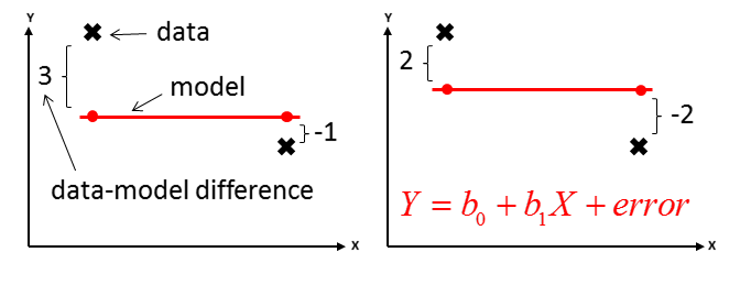
Hypothetical data points and model. The sum of the absolute distances is the same for both, the distance squared favors the model on the right.

Mathematically, the equation for the sum of squares can be written as \(SS=\sum_i \left(\textrm{data}_i - \textrm{model}_i \right)^2\). The index i runs over all datapoints. We try to find a model that makes this quantity as small as possible.

Alternative names for the sum of squares quantity are sum of square residuals, residual some of squares, residual sum error and similar. Mean squared error (MSE) is an equivalent metric, with the difference that we divide by the sample size, i.e. MSE=SS/N. Similarly, the root mean squared error (RMSE), is just the square root of the MSE. For a given dataset, minimizing any of these quantities is the same as they only differ by some factor that does not depend on the model. Note however that you cannot compare SS for different datasets. Using MSE and RMSE to compare different samples of the same dataset is often done, but requires caution. Using those metrics to compare across completely different datasets is generally not valid.

Manual least squares fitting

Let’s try another fitting exercise where we manually try to find the best model, now with the help of the SSR equation. The following shows both the plot and prints the sum of square residuals (SSR) to the screen. See how SSR changes as you change the model parameters.

Notice the issue mentioned previously: Among those 4 choices, the parameter combination that produces the lowest SSR doesn’t actually make sense, since the intercept should be 0. What does a negative intercept even mean? If the car travels at no speed, it takes negative distance to stop? Of course the model does not know the meaning of the variables, and given that there are is noise/scatter in the data, just tries to get as close as possible, given the model and the metric/objective function. Deciding if a statistical result makes sense is up to you, the analyst.

Automated least squares fitting

Of course, we don’t want to fit models by hand. Also, if we have multiple predictors, we can’t properly visualize the model fit anymore. Fortunately, the general approach still works, no matter how many predictors we have and what type of model we fit. The general approach is:

• Decide on the kind of model you want to fit. Based on the model choice, it will have some parameters that need to be chosen. For a (generalized) linear model, those are the coefficients in front of the predictor variables. Other types of models will have different parameters that can be adjusted (tuned) during the model fitting (training) process.
• Decide on the metric/cost function you want to optimize. Here, we are using sum of squares (SSR) and minimizing it. But this applies for any metric.
• Choose some starting values for the model parameters you plan on adjusting, run model, compute your metric by comparing model predictions and actual outcomes.
• Change model parameters, repeat.
• Continue adjusting the model parameters until you found the best value for your metric, here the smallest possible SSR.

We’ll let the computer do this process. If we want to fit a linear model, we can use the lm function in R. Write a line of code that fits distance to standstill as function of speed using the lm function, and saves the answer in an object variable called fit1. Then use the summary() function to get all kinds of information about the fit. Compare those results to the information you get when you print the fit1 object to the screen using the print() command.

Note that you should use base R commands here. Depending on what server you run this from, tidyverse or tidymodels packages might not be installed/available. Also, it’s good to know how to do basic computations with standard R functions, even if for most of your real data analysis projects you prefer using functions that come with specific R packages.

# Write code that fits a linear model of distance vs speed and looks at the results 

fit1 <- lm(cars$dist ~ cars$speed)
summary(fit1)
print(fit1)

The summary command gave you the residual standard error (RSE) and \(R^2\). Let’s compute those 2 by hand and make sure things agree.

Write code to compute \(R^2\) yourself and compare that value with the one provided by the summary function. There are different ways of doing it, let’s do it the most explicit way so you can see each step, and get an idea how this can be applied in general. First, store the outcomes in the data (the distance to stop) in a variable out_dat, and compute the mean of the outcomes and store it in a variable out_mean. Then use the predict() function to get model predictions for the outcomes and store that in a variable out_pred.

Then use the SSR equation to compute sum of squares and the SST equation to compute the sum of square totals. Then use SSR and SST to compute \(R^2\). You can look at the course readings for details, or check this Wikipedia article. What I call SSR and SST here, they call SSres and SStot.

Once you got all the quantities computed, print SSR and \(R^2\) to the screen and compare with values you got from the summary() function. They should agree.

fit1 <- lm(cars$dist ~ cars$speed) #we need to repeat that so it's available
#write code that computes SSR and R-squared

fit1 <- lm(cars$dist ~ cars$speed) #we need to repeat that so it's available
out_dat <- cars$dist
out_mean <- mean(cars$dist)
out_pred <- predict(fit1)
SSR <- sum( (out_pred - out_dat)^2 )
SST <- sum( (out_mean - out_dat)^2 )
R2 <- 1 - SSR/SST
print(SSR)
print(R2)

Almost always, you do not need to compute standard quantities like this by hand. But it is good to know how you could do it. There might be instances where you need it. Let’s say we knew that for any car that had a speed over 15, the distance measure was less reliable as for the cars that drove slower, and we want to put weights on that by multiplying the (data - model)^2 values in the SSR computation by 0.5 for those cars with speed over 15. Basically, this means creating a custom metric. Packages like tidymodels allow you to specify custom metrics. To do so, you need to supply some lines of code that compute the different components, similar to what you just wrote. Thus, it is useful to know how to compute those metrics yourself, even if you end up doing so very rarely.

Beyond ordinary least squares

Simple/ordinary least squares is often a good choice as the metric to use for continuous outcomes, and by far the most widely used. But sometimes, other metrics might be better. We’ll briefly explore a least absolute deviation fit. For absolute deviation, the metric you are minimizing the sum of absolute differences between model predictions and data, i.e. \(\sum_i|d_i-m_i|\) instead of the squared differences between model predictions and data for least squares (\(\sum_i (d_i-m_i)^2\)). Here \(d_i\) and \(m_i\) are all outcomes in the data and all model predicted outcomes respectively.

fit2 <- rq(cars$dist ~ cars$speed)
summary(fit2)
print(fit2)

The summary() function applied to fit2 does not give you an \(R^2\) value. That kinda makes sense, since we didn’t actually work with SSR and SST. But let’s say for some reason we still wanted to determine the \(R^2\) value. Luckily, you just learned how to compute it yourself. Write some code to compute it, similar to the code you just wrote above.

fit2 <- rq(cars$dist ~ cars$speed)
#write code that computes SSR and R-squared

fit2 <- rq(cars$dist ~ cars$speed)
out_dat <- cars$dist
out_mean <- mean(cars$dist)
out_pred <- predict(fit2)
SSR <- sum( (out_pred - out_dat)^2 )
SST <- sum( (out_mean - out_dat)^2 )
R2 <- 1 - SSR/SST
print(SSR)
print(R2)

Some additional comments

You might be wondering why the summary() function produces different answers for fit1 and fit2. That has to do with the fact that the function looks at the kind of object/variable that is being sent to it (here fit1 and fit2) and depending on the type/class of object, will deploy a different underlying summary() function written specifically for that object.

If you look at the help file for the summary() function, you will see it states that it’s a generic function. What that essentially means is that it is a convenience function that you can call, the function looks at the type of object you provide, and then calls the actual function doing the work appropriate for the task, based on the class of the object. In R you can check what object class a variable is with the class() command. Here, the class of fit1 is lm, the class of fit2 is rq. You can call the summary functions that go with each object directly, with summary.lm(fit1) and summary.rq(fit2). You will get the same answer as when you use summary. If you try to send fit1 to summary.rq or the reverse, you will get error messages.

R has several such generic functions which look at the object that is supplied and then perform different actions, examples are plot and print. The good thing is that you have to learn fewer commands and can apply them to different objects. The bad thing is that the person writing each specific function decides how their function operates. In the above example, summary.lm gives you \(R^2\) while summary.rq does not. That’s where frameworks like tidymodels become useful. They allow you to switch between models and underlying statistical fitting packages/functions without having to do major rewriting of your code. Therefore, for most full analyses, using the extra layer of going through e.g. the tidymodels framework is worth it.